Data analysis with numpy, datascience and matplotlib: Curve fitting
Objectives for today
Use the numpy, datascience and matplotlib libraries
Apply a variety of methods for generating a line of best fit
Translate mathematical expressions into Python code
As quick reminder, here are the standard set of imports we are using (note that the order matters, datascience needs to be imported before matplotlib):
import numpy as npimport datascience as dsimport matplotlibmatplotlib.use('TkAgg')import matplotlib.pyplot as plt
How far can you make a paper airplane fly?
In class, you’ll work in groups of 2-3 to make your own paper airplane from a single letter-sized 8.5x11” sheet of paper. The goal is to make the plane fly as far as possible (take about 5 minutes to do this).
Expand to see some options
Fitting a line
When you were making your paper airplane, you may have tried to maximize the wing area or the length of the wings. This might lead to a longer flight distance because this type of design might generate more lift (the force that pushes your airplane upwards). More lift could mean your airplane stays in the air a bit longer, so it will probably fly a longer distance.
Let’s start with this script to analyze some paper airplane data. Note that we can load a dataset directly from the internet. We currently have the following dataset (which contains some made-up values):
# Load data as datascience.Table directly from the Internetdata = ds.Table.read_table("https://philipclaude.github.io/csci146f25/classes/paper-airplane-data.csv")data
Wingspan
Distance
8
2.84
10
5.3
12
5.52
14
7.3
16
7.84
18
9.24
20
8.5
22
9.52
24
8.3
26
8.84
... (1 rows omitted)
During class, I’ll update this Google spreadsheet with our experimental results. We’ll then include it in our analysis:
sheet_name ="PaperAirplaneExperiment"sheet_url ="https://docs.google.com/spreadsheets/d/1t4GBPuhqjnxeNWBHBy1gRUsmkmW86MEn3OmSD-L4Cyo/gviz/tq?tqx=out:csv&sheet="+ sheet_nameexperimental_data = ds.Table.read_table(sheet_url)print(experimental_data)# data.append(experimental_data) # uncomment to include in-class experiment data
# Generate a scatter plot with `Wingspan` as the x-axis and `Distance` as the y-axisdata.scatter("Wingspan", fit_line=True)plt.ylabel("Distance [m]")plt.xlabel("Wingspan [cm]")plt.show()
Where did that line come from? It is the “line of best fit”, which is the line that minimizes the mean squared error (MSE) between the fitted or predicted values and the actual values. That line is also the “regression line”, i.e, the line that predicts the flight distance as a function of wingspan. The different names for that line give some ideas for how we could compute that line for ourselves:
Determine the regression line
Determine the line of best fit by minimizing mean squared error (MSE)
Using existing library functions for fitting
Regression line
The following describes the slope and intercept for simple linear regression, i.e., a linear regression model with one independent or “explanatory” variable, \(x\), and one dependent variable, \(y\):
where \(\bar{x}\) and \(\bar{y}\) are the means of the \(x\) and \(y\) values, respectively. Let’s implement this calculation as a function regression_line that returns the slope and intercept of the regression line as a numpy array.
TipWhere did the slope and intercept come from? (optional)
The slope and intercept are derived from the correlation coefficient, \(r\), of the two variables, \(x\) and \(y\). Specifically: \[
\begin{align*}
\text{slope} &= r\cdot \frac{\text{SD of }y}{\text{SD of }x} \\
\text{intercept} &= \bar{y} - \text{slope} \cdot \bar{x}
\end{align*}
\]
The correlation coefficient, \(r\), is a measure of the strength and direction of a linear relationship between two variables. The correlation coefficient ranges from -1 to 1, with 1 indicating a perfect positive linear relationship, -1 indicating a perfect negative linear relationship, and 0 indicating no linear relationship. \(r\) is calculated as the average of the product of the two variables, when they are transformed into standard units. To transform a variable into standard units, we subtract the mean of the variable and divide by the standard deviation. Plugging that into the definition of \(r\) gives:
\[
r = \frac{\sum_{i=1}^{N} \frac{(x_i - \bar{x})}{\text{SD of }x}\frac{(y_i - \bar{y})}{\text{SD of }y}}{N}
\]
We can now express the slope as \[
\begin{align*}
\text{slope} &= r\cdot \frac{\text{SD of }y}{\text{SD of }x} \\
\text{slope} &= \frac{\sum_{i=1}^{N} \frac{(x_i - \bar{x})}{\text{SD of }x}\frac{(y_i - \bar{y})}{\text{SD of }y}}{N} \cdot \frac{\text{SD of }y}{\text{SD of }x} \\
\text{slope} &= \frac{\sum_{i=1}^{N} \frac{(x_i - \bar{x})}{(\text{SD of }x)^2}(y_i - \bar{y})}{N} \\
\text{slope} &= \frac{\sum_{i=1}^{N} \frac{(x_i - \bar{x})N}{\sum_{i=1}^N (x_i - \bar{x})^2}(y_i - \bar{y})}{N} \\
\text{slope} &= \frac{\sum_{i=1}^{N} (x_i - \bar{x})(y_i - \bar{y})}{\sum_{i=1}^{N} (x_i - \bar{x})^2}
\end{align*}
\]
Minimizing mean squared error
We can also describe the line of best fit as the line that minimizes the mean squared error (MSE) between the fitted values and the actual values. We can perform that minimization by defining a function that calculates the MSE for a given slope and intercept and then using tools in Python’s scientific libraries to find the arguments that minimize the return value of that function. Specifically we can use the minimize function in the datascience library (which is a wrapper around the minimize function in the scipy library).
Let’s start by writing a function fit_mse that takes two parameters, slope and intercept and returns the MSE between the fitted values and the actual values, assuming the input and output data are stored in the variables x and y, respectively. We can then use this function as the argument to the minimize function. minimize will run this function with different values of slope and intercept until it finds the values that minimize the MSE.
We didn’t define where x and y will come from. Wrap your definition of fit_mse in a function mse_line that takes the input data x and y and returns the result of minimize on fit_mse. Doing so creates a nested function that has access to the variables x and y that were defined when the function was created (often called a closure). We have generally discouraged the use of nested functions in this course, but they can be useful in certain situations like this one. Here the inputs slope and intercept change during the minimization, while x and y remain fixed. We define the former as the function parameters, and “embed” the latter in the nested function.
def mse_line(x, y):# Create a nested function that takes the parameters to minimize while "closing"# over (embedding) the current x and y values. We can then call this function without# needing to pass x and y as arguments.def fit_mse(slope, intercept): fitted = slope * x + interceptreturn np.mean((y - fitted) **2)# Use the minimize function to find the parameters that minimize the output the# the function passed as an argumentreturn ds.minimize(fit_mse)
We can then apply this function to the flight data to determine the line that minimizes the MSE. As expected, we get the same slope and intercept as the regression line (within the limits of numerical precision)!
datascience.minimize provides a convenient wrapper around the scipy.optimize.minimize function that handles initial values, splitting the parameters into separate arguments, etc. We could also use scipy.optimize.minimize directly, with small changes.
Here we define a function scipy_fit_mse that takes the parameters to minimize as an array. We further specify the x and y arrays as additional argument. We will pass those arrays through minimize so we don’t need to create a nested function with those values “embedded” (“closed” over). We then use that function as the argument to minimize, also passing the initial values as the x0 parameters, and a tuple of x and y as the args parameter. minimize will pass the values in the args tuple through as the additional arguments to the function it is minimizing (scipy_fit_mse in this case).
import scipy.optimize as opt# Define a function that takes the parameters to minimize as an array, and the x and y arrays# as additional argumentsdef scipy_fit_mse(params, x, y): fitted = params[0] * x + params[1]return np.mean((y - fitted) **2)def scipy_mse_line(x, y):# Use the minimize function to find the parameters that minimize the output of the function# provided as the first argument. x0 is the initial values. We pass the x and y arrays as a tuple# in the args parameter, which will be passed through to the function as additional arguments (it# becomes the x and y parameters above). result = opt.minimize(scipy_fit_mse, x0=[0, 0], args=(x, y))return result.xscipy_mse_line(data["Wingspan"], data["Distance"])
array([ 0.23681812, 3.09545573])
Using library functions
We would imagine that fitting a line is a common task, and thus Python’s scientific libraries should already have functions that do this. Indeed, the numpy library has a np.polyfit function that fits a polynomial of a given degree to the data. We can use this function to fit a line to the flight data.
# Fit a line to the data return parameters as an array, in descending order of degree, e.g.,# [slope, intercept] for a linepline = np.polyfit(data["Wingspan"], data["Distance"], 1)pline
array([ 0.23681818, 3.09545455])
When we apply this function to the flight data we get the same effective slope and intercept as before (if we didn’t, we would have to check our work). We can then plot this line on top of the scatter plot of the data using the axline function in matplotlib. That function plots an a line given a point and a slope (or two points).
It doesn’t really look like a straight line fits the data very well. Let’s extend our previous approaches to fit a quadratic function to the data. Recall that the general form of a quadratic function is
\[y = ax^2 + bx + c\]
We can apply a similar approach to finding the quadratic function that minimizes the mean squared error between the fitted values and the actual values. Write a function mse_quadratic that takes the input data x and y and uses minimize to fit a quadratic function to the data. The approach is similar to the linear case, but the implementation for the nested fit_mse function changes.
def mse_quadratic(x, y):# Now fit a quadratic function, i.e., a*x^2 + b*x + c, with 3 parametersdef fit_mse(a, b, c): fitted = a * (x**2) + b * x + creturn np.mean((y - fitted) **2)return ds.minimize(fit_mse)
We can then apply this function to the flight data. We can also use the np.polyfit function to do the same, increasing the degree of the polynomial to 2 to fit a quadratic function. As expected, we get the same parameters for both approaches (within the limits of numerical precision).
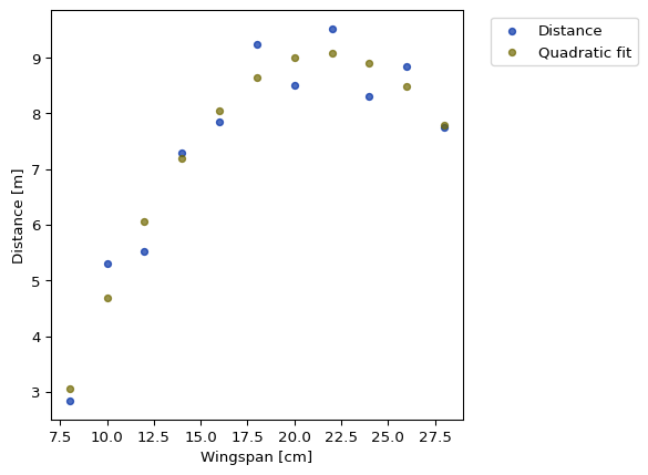
With those fits we can plot the quadratic fit on top of the scatter plot of the data. Here we generate fitted values for the same “x” values as the data and plot those as a second series with the scatter method.
flight_fit = pquad[0]*(data["Wingspan"]**2) + pquad[1]*data["Wingspan"] + pquad[2]# Create a new table with fitted values added as a column, plotting both vs. "Wingspan"data = data.with_column("Quadratic fit", flight_fit)data.scatter("Wingspan")plt.ylabel("Distance [m]")plt.xlabel("Wingspan [cm]")plt.show()
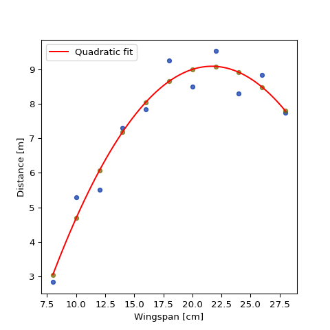
That plot approach makes it difficult to interpolate the fitted values. Instead we would like to plot the fitted curve. Unfortunately there aren’t built functions for plotting quadratic curves from their parameters (as we did the linear line above). Instead we can generate a range of x values and plot the fitted curve over that range as a line plot. Below we use the np.linspace function to generate an array of equally spaced values over the range observed in the data, then compute the expected outputs for those values.
data.scatter("Wingspan")# Generate "curve" over the range of the data by creating linear spaced "x" values and c# computing the fitted valuesx = np.linspace(data["Wingspan"].min(), data["Wingspan"].max(), 100)flight_fit = pquad[0]*(x**2) + pquad[1]*x + pquad[2]plt.plot(x, flight_fit, color="red", label="Quadratic fit")plt.ylabel("Distance [m]")plt.xlabel("Wingspan [cm]")plt.legend()plt.show()
This seems to capture the flight data a bit better. And it physically makes sense too. The linear fit implied that we could make the wings infinitely long to make the paper airplane fly a super long distance. But that won’t really happen in real life. At some point, the increase in wingspan (and wing area, and probably weight too) will create more drag on the wing (the force that opposes the motion of the airplane), which will cause a shorter flight.