Class 16

Complexity analysis (big-O), numerical representation

Objectives for today

Informally define asymptotic complexity with a focus on runtime
Describe the purpose and calculation of Big-O notation
Compare (e.g. rank) constant, logarithmic, linear, quadratic, and cubic complexities
Predict the runtime of an algorithm based on its Big-O complexity
Explain how integers and other types are represented in the computer
Perform binary addition of unsigned integers
Be aware of twos-complement representation
Be aware of the floating point representation and some of its limitations

Revisiting list vs. set

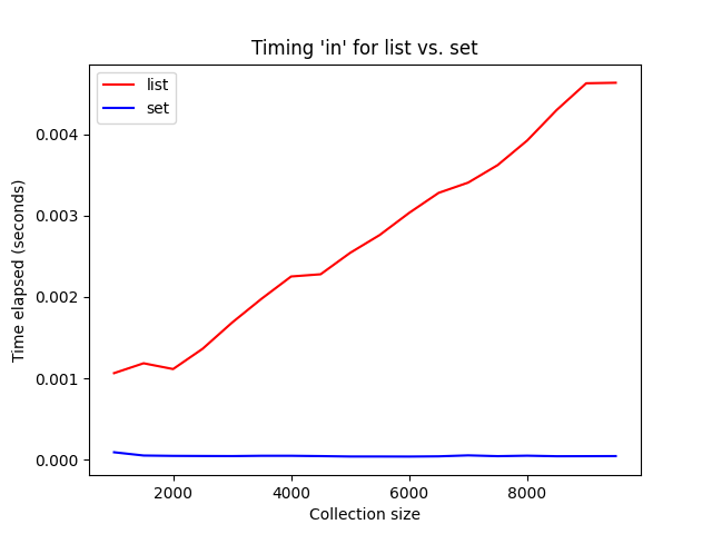
Several classes ago, we plotted the execution time of membership queries of list and sets of different sizes. Recall that we observed that the query time grew linearly with the size of list, but did not grow at all as we increased the size of the set:

Today we are going to talk more formally about how to analyze the efficiency of these and other algorithms.

Introducing big-O

We can always talk about absolute running time, but that requires lots of experimentation and is easily confounded by different inputs, the particular computer we are using, etc. Instead we want a tool that allows us to talk about and compare different algorithms, data structures, etc. before we do any implementation, while eliding unnecessary details.

That tool is asymptotic analysis, that is an estimate of the execution time (termed time complexity), memory usage or other properties of an algorithm as the input grows arbitrarily large.

The key idea: How does the run-time grow as we increase the input size? For example, in the case of querying lists, if we double the size of the list, how will the execution time (time complexity) grow? Will it be unchanged, double, triple, quadruple? Double! Similarly, how would the execution time of querying sets grow if we double the size of the set? Unchanged!

Big-O notation is way of describing the upper-bound of the growth rate as a function of the size of the input, typically abbreviated n. That is, it is really about growth rates. Big-O is a simplification of \(f(n)\), the actual functional relationship, which follows these two rules:

If \(f(n)\) is the sum several terms, only the term with largest growth rate is kept.
Any constant terms, i.e. those that do not depend on n are omitted.

Thus \(f(n)=3n^3 + 6n^2 + n + 5\) would be \(O(n^3)\).

Using big-O, we can describe groups of algorithms that have similar asymptotic behavior:

Complexity	Description
\(O(1)\)	Constant
\(O(\log n)\)	Logarithmic
\(O(n)\)	Linear
\(O(n\log n)\)	Linearithmic
\(O(n^2)\)	Quadratic

Returning to our “list vs. sets” example, querying a list is \(O(n)\) or linear time and querying a Python set is \(O(1)\), or constant time.

Using and determining big-O

Suppose that we had an algorithm with \(O(n^2)\) complexity that takes 5 seconds to run on our computer when n is 1000. If the input increased to n of 3000, about how long would it take to run?

Show an answer

Since we are tripling the input, and the algorithm has quadratic complexity, the time will grow as \(3^2\), or by a factor of 9. Thus we would expect it to take 45 seconds with the larger input.

What about the standard deviation computation in our programming assignment? Two possible implementations are shown below:

def mean(data):
    """
    Return mean of iterable data
    """
    return sum(data) / len(data)
    
def stddev(data):
    """
    Return standard deviation for iterable data
    """      
    result = 0.0
    average = mean(data)
    for elem in data:
        result += (elem - average) ** 2
    return math.sqrt(result / (len(data) - 1))
    
def stddev2(data):
    """
    Return standard deviation for iterable data
    """      
    result = 0.0
    for elem in data:
        result += (elem - mean(data)) ** 2
    return math.sqrt(result / (len(data) - 1))

What is the complexity of these two implementations?

Show an answer

In the first, we compute the mean before the loop. Thus inside the loop we are only performing a constant number of operations (a subtraction, multiplication and addition). Thus it is a linear time implementation. In the latter, in each loop iteration, i.e. n times, we are computing the average, an \(O(n)\) operation. Thus the overall complexity is \(O(n^2)\), or quadratic! We should choose the first approach!

So thinking back to the choice between a list and a set for querying, should we always choose the set because its time complexity is better? It depends. Keep in mind that big-O approximates the growth rate in the limit where the input size is very large. So if the inputs are large then we would almost certainly want to choose a set. If that assumption does not hold for our input, e.g., we are querying just a few values, then the set may not be any faster.

And also keep in mind that big-O drops the constants, however in reality the constant factors may be quite large. Thus think of big-O as a useful tool for thinking about efficiency (albeit with caveats) that complements experiments and other approaches.

What is an operation?

We have determined the big-O for algorithms by counting operations, e.g., addition, multiplication, etc. What do those operations actually entail? How do we actually add on a computer? That is our next topic (and a preview for CS202).

Representing numbers in binary

What is created when you type the following, that is how does Python represent integers?

>>> x = 17

Recall that everything in Python is an object so when evaluating the RHS, Python allocates an int object, stores 17 within that object and then sets x to point to that object.

But that hasn’t answered our question of how “17” is represented. Although you might reasonably guessed, since computers are built from binary (digital) logic, it is somehow represented in binary.

As an aside, why binary? Because we can easily represent binary values and implement boolean logic with transistors, that is logical operations over values of 0 and 1 (corresponding to 0 volts and “not 0” volts), but it is trickier to represent numbers with more levels.

Let us first remind ourselves what “17” represents. We typically work in base-10, i.e. the first (rightmost) digit represents numbers 0-9, then the second digit, the tens, represents 10, 20, etc. and so on. That is the contribution of each digit is

\[base^{index}*value\]

or 1*10 + 7*1.

The same notion applies to binary, that is base-2 numbers. Except instead of the ones, tens, hundreds, etc. place, we have the ones, twos, fours, eights, sixteens, etc. place.

So 17 in binary notation is 10001 or 1*16+1*1. We often call each of these binary digits, i.e., each 0 or 1, a “bit”. So 10001 is 5 “bits”.

Python has a helpful built-in function bin, for generating a binary representation of a number (as a string). The 0b prefix indicates that this is a binary (or base-2) number (not a base-10 or decimal number). We should note that the resulting string is close to, but not identical, with how Python actually represents integers in memory. You will learn those details in CS202.

bin(17)

'0b10001'

Converting between binary and decimal

Converting from binary to decimal can be done with \(base^{index}*value\). As we saw earlier, 10001 is 1*16+1*1. Converting from decimal to binary (by hand) is a little more laborious. We can do so by iteratively subtracting the largest power of two that is still less than our number. Consider 437 as an example:

 437
-256  # 256 is highest power of 2 less than 437
----
 181

 181
-128  # 128 is highest power of 2 less than 181
----
  53

 53
-32   # 32 is highest power of 2 less than 53
---
 21

 21
-16   # 16 is highest power of 2 less than 53
---
  5

437 = 256 + 128 + 32 + 16 + 4 + 1 or 2^8 + 2^7 + 2^5 + 2^4 + 2^2 + 2^0 or 110110101

Binary arithmetic

We can add binary numbers just like we do decimal numbers. Think back to how you did it in elementary school… Start at the right most digits, add, if the sum is greater than or equal to the base, carry the one. Then repeat for every digit. Consider the following example for 23 + 5:

  111
 10111
+00101
------
 11100

>>> bin(23)
'0b10111'
>>> bin(5)
'0b101'
>>> bin(28)
'0b11100'

Same with subtraction… Start with the right most digit, if the top digit is greater, subtract the digits, the bottom digit is greater “borrow” 1 from higher digit. Consider the following example for 17 - 10:

 10001
-01010
------
     1

    1 
 01111
-01010
------
 00111

Here we need to borrow from the 16s place into the 2s place.

>>> bin(17)
'0b10001'
>>> bin(10)
'0b1010'
>>> bin(7)
'0b111'

Why does this matter?

The limitations (and the capabilities) of the underlying representation will impact our programs. For instance, can we represent all integers? Yes and no. There are maximum and minimum integers.

import sys
sys.maxsize

9223372036854775807

Does that mean we can’t work with larger integers? No. Python transparently switches the underlying representations when integers grow beyond the “natural size” of the computer. This is actually an unusual feature. Most programming languages have a maximum representable integer (and then require you to use a separate library for larger numbers). The NumPy library, which we talk about soon, is much more tied the underlying capabilities of the computer and so has a stricter maximum integer. There are also performance implications to exceeding the natural size.

“Natural” size and negative numbers

The maxsize number we saw above may seem arbitrary. But it is not:

(2**63)-1

9223372036854775807

I have a 64-bit computer (i.e., the natural size of an integer is 64 binary digits), why is the natural size (2^63)-1? Shouldn’t it be (2^64)-1? The difference results from how we represent negative numbers. Specifically computers use a scheme known as two’s-complement to encode negative and positive numbers. While we could just use the highest order bit to indicate sign, that creates two zeros (positive and negative) and makes the math hard. In contrast with two’s complement, we don’t have to change anything about the math. For example, 17 + -10:

 1
 010001
+110110
-------
 000111

Using two’s-complement requires a fixed length. We can then convert from one’s-complement by inverting all bits and adding one.

In this class we are not concerned with the details of two’s complement, but I do want you to be aware that this approach is used to implement negative numbers (and thus why the maxsize is the way it is).

Floating point numbers

The subtleties of floating point computations are similarly beyond the scope of this course, but as with two’s-complement, I want you to be aware that such subtleties do exist. Thus hopefully any non-intuitive behavior you observe will not be a surprise. As we discussed very early in the course floats have finite precision and thus can’t represent all real numbers. As a result we can observe behavior that deviates from the results we would otherwise expect from a mathematical perspective. Recall our previous curious example:

0.1 + 0.2 <= 0.3

False

To understand what is going on we can use the Python decimal module, which implements exact representations of decimal numbers. We can see that the results of the addition are a float slightly larger than 0.3 and the literal 0.3 is translated into a float slightly less than 0.3. As a result our comparison produces incorrect results!

import decimal
decimal.Decimal(0.1 + 0.2)

Decimal('0.3000000000000000444089209850062616169452667236328125')

decimal.Decimal(0.3)

Decimal('0.299999999999999988897769753748434595763683319091796875')

Floating numbers are implemented as

\[sign*1.mantissa*2^{exponent-\textrm{bias}}\]

For the 64-bit “double precision” floating point numbers used by Python, the sign is one bit, the “exponent” is 11 bits and the “mantissa” (also called the “significand”) is 52 bits (creating 53 bits of effective precision because of the implicit leading 1). That is sufficient for 15-17 significant digits in a decimal representation.

What does this mean as a practical matter for us? We should be aware of the limited precision. Equality comparison of floating point numbers is fraught (as we saw above) and so if we need to perform such a comparison, we should use equality within some tolerance (what all of our Gradescope tests do). With the limited range (see below) we can have overflow - numbers too large to represent - and underflow - numbers too small to represent. The latter can arise, for instance, when multiplying many small probabilities. As a result you will sometimes see computations performed in log-space (so small numbers become large negative numbers and multiplication becomes addition).

import sys
sys.float_info

sys.float_info(max=1.7976931348623157e+308, max_exp=1024, max_10_exp=308, min=2.2250738585072014e-308, min_exp=-1021, min_10_exp=-307, dig=15, mant_dig=53, epsilon=2.220446049250313e-16, radix=2, rounds=1)

And if we are performing computations that require exact decimal values, e.g. financial calculations, we should use modules like decimal that are specifically designed for that purpose.

Class 16

Objectives for today

Revisiting list vs. set

Introducing big-O

Using and determining big-O

Other types of problems

Traveling salesperson problem

Undecidable problems

What is an operation?

Representing numbers in binary

Converting between binary and decimal

Binary arithmetic

Why does this matter?

“Natural” size and negative numbers

Floating point numbers