def power(base, exp):
if exp == 0:
return 1
else:
y = power(base, exp//2)
return y * y
power(2, 7) # Should be 1281Recursion, cont.
turtle.lenLet’s write a recursive function named rec_len that takes a non-empty sequence as a parameter and returns the number of items in the sequence. Following our 4 step process:
Specify the function definition: rec_len(seq)
Specify the recursive relationship
In a previous class we discussed techniques for making the problem get “smaller”, including approaches that split a sequence (such as a list or string) into its first element and the rest of the sequence. Using that idea, we could express the recursive relationship as: the number of elements in a sequence is 1 plus the number of elements in the rest of the sequence.
Specify the base case
The smallest version of the problem is an empty sequence, which has 0 elements. To avoid using the len function, we can take advantage that empty sequences are “falsy”, i.e., treated as False.
Put it all together.
def rec_len(seq):
    """ Return the number of items in seq """
    if not seq:
        return 0
    else:
return 1 + rec_len(seq[1:])Consider the following code to draw a spiral. In each iteration it draws a segment, turns left, and then recursively draws shorter segments (only 95% of the length).
import turtle as t

def spiral1(length, levels):
    """
    Draw a spiral with 'levels' segments with initial 'length'
    """
    # Implicit base case: do nothing if levels == 0
    if levels > 0:
        t.forward(length)
        t.left(30)
        spiral1(0.95 * length, levels-1) # Recurse
Try running the code with say, spiral1(80, 45). Notice that the turtle stops and remains where the drawing ends at the inner tip of the spiral.
Let’s revise this code to “undo” the calls to forward and left with “pending operations”. After the recursive call to spiral2(0.95 * length, levels-1), undo the left turn by turning right, and undo the forward by moving backward:
import turtle as t

def spiral2(length, levels):
    """
    Draw a spiral with 'levels' segments with initial 'length'
    """
    # Implicit base case: do nothing if levels == 0
    if levels > 0:
        t.forward(length)
        t.left(30)
        spiral2(0.95 * length, levels-1) # Recurse
        t.right(30)
        t.backward(length)
If we started with the turtle at (0,0), what is the position of the turtle after invoke this function, e.g. spiral2(80, 45)? The turtle ends up back at (0,0) because we are “retracing” the movements after the recursive call. This is a common pattern in recursive functions in which we “reset” the state after a recursive call using pending operations and state maintained in the call stack.
How can we draw the following trees recursively?
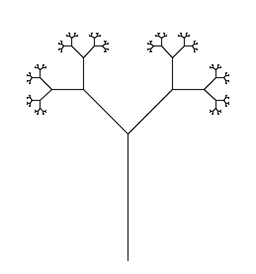
We might be able to do this with a for-loop, but notice that each junction in the tree starts a new tree, so recursion might be a good idea here. We also need to identify what our recursion variable is. In this case, we have two options: we can either use the length of the trunk/branch to draw for the current tree, or we can use the idea of “levels”. The trunk length might be more natural for now, but we’ll come back to the idea of levels soon.
Thinking about our four steps:
Specify the function definition: draw_tree(length)
Specify the recursive relationship.
When we’re in the recursive step, we want to do two things. First, we’ll advance the turtle to draw the trunk. Then we’ll turn the turtle to draw two subtrees (which we’ll do recursively). The angle we’ll use to turn will be 45 degrees (left and right), but we can also use different angles if you want. After the subtrees are drawn, we’ll retreat back to the base of the trunk (of the current subtree).
Specify the base case.
When the input length is zero, we want to stop drawing. We can also terminate drawing a little sooner if we don’t want to draw really tiny subtrees.
Put it together.
Here’s a possible implementation. I would suggest turning the turtle left by 90 degrees and then calling draw_tree(128).
def draw_tree(length):
"""
Draw a recursive tree and return to where the turtle started
Args:
length: length of initial tree trunk
"""
if length > 0:
t.forward(length) # draw tree branch
t.right(45)
draw_tree(length // 2) # draw right subtree
t.left(45*2) # undo right turn, then turn left again
draw_tree(length // 2) # draw left subtree
t.right(45) # undo left turn
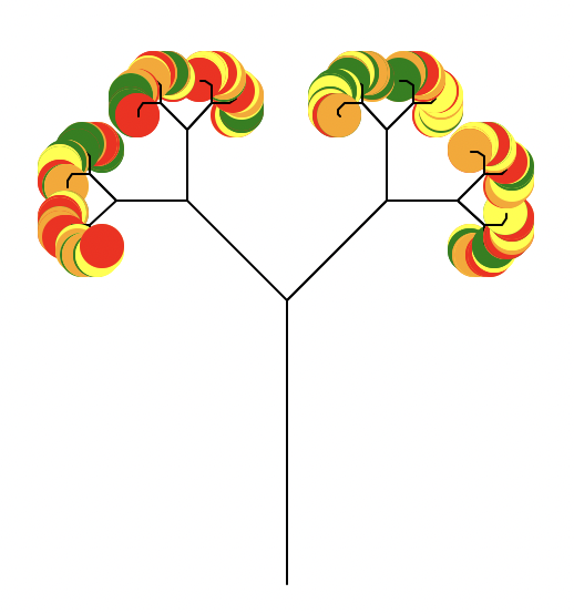
t.backward(length) # trace back down the tree branchThe above function draws nothing if levels is 0. This is another example of an “implicit base case” that simply returns (terminating execution) without doing anything. If you want you can change the base case to draw leaves:
import random
COLORS = ["red", "green", "orange", "yellow"]

def draw_tree(length):
    """
    Draw a recursive tree and return to where the turtle started
    Args:
        length: length of initial tree trunk
    """
    if length > 0:
        t.forward(length)           # draw tree branch
        t.right(45)
        draw_tree(length // 2)      # draw right subtree
        t.left(45*2)                # undo right turn, then turn left again
        draw_tree(length // 2)      # draw left subtree
        t.right(45)                 # undo left turn
        t.backward(length)          # trace back down the tree branch
    else:
        # draw fall-like leaves at the end of the tree
        color = COLORS[random.randint(0, len(COLORS) - 1)]
        t.pencolor(color)
        t.fillcolor(color)
        t.dot(20)
        t.pencolor('black')
Let’s come back to this concept of “levels” and write some code to help us visualize these levels. The level refers to how many branches have been traversed to get from the base of the tree (or root) to the current location. We’ll extend our draw_tree function to now accept a second parameter called level which will be defaulted to 0 when draw_tree is first called and will be incremented as we move up the tree. We can also use the turtle.write method to write the current level of the (sub)tree at the current turtle location. You might want to comment out the drawing of leaves to make this clearer.
def draw_tree(length, level=0):
    """
    Draw a recursive tree and return to where the turtle started
    Args:
        length: length of initial tree trunk
        level: current level (# branches from root to current location)
    """
    if length > 0:
        t.forward(length)                   # draw tree branch
        t.right(45)
        draw_tree(length // 2, level + 1)   # draw right subtree
        t.left(45*2)                        # undo right turn, then turn left again
        draw_tree(length // 2, level + 1)   # draw left subtree
        t.right(45)                         # undo left turn
        t.backward(length)                  # trace back down the tree branch
        t.write("L" + str(level), align="center")
We’re actually drawing something called a binary tree which shows up a lot in computer science. Binary trees are covered in detail in CSCI 201 (Data Structures).
Let’s relate the length drawn at each level from t.forward(length) with the current level number. For the first branch (the trunk) we draw a length of length (level 0). The second branch has a length of length/2 (level 1). The third branch has a length of (length/2)/2 = length/4 (level 2). The fourth branch has a length of (((length/2)/2)/2) = length/8 (level 3). Hmm. It kind of looks like there’s a “power-of-2” relationship between the level and the length of the current branch to draw:
\[ 2^{\texttt{level}} = \texttt{length}. \]
The last line drawn has a length of 1, which corresponds to \(\texttt{level} = \log_2(\texttt{length})\). The leaves (the base case) are one additional level from this, so the final level is \(\texttt{level} = \log_2(\texttt{length}) + 1\). This type of analysis will be useful as we talk about the efficiency of recursive functions.
Let’s develop a recursive implementation for power, with parameter base and exp (exponent). Using our 4 step process:
Define the function header, including the parameters
def power(base, exp)Define the recursive case
\[\mathrm{base}^{\mathrm{exp}} = \mathrm{base} * \mathrm{base}^{(\mathrm{exp}-1)}\]
Define the base case
\[\mathrm{base}^0 = 1\]
Put it all together
def power(base, exp):
    if exp == 0:
        return 1
    else:
        return base * power(base, exp - 1)
How many times are we calling power(base, exp)? exp + 1 times (the +1 comes from the first call). This also relates to how much memory our program will use because Python will need to create a new frame in the call stack for each call to power.
Can we do better? Yes!
Note that \(\mathrm{base}^{\mathrm{exp}}=\mathrm{base}^{\mathrm{exp}/2}*\mathrm{base}^{\mathrm{exp/}2}\). So what if instead of recursing by exp-1, we recursed by exp/2 (dividing in half)? How many calls to power are done in that case? To answer this question, think about how many times we need to divide exp/2 until we reach the base case. Our base case is exp == 0, but let’s focus on how many calls to power it takes to get to exp == 1. Let p be the number of calls to power:
\[ \frac{\texttt{exp}}{2^p} = 1 \quad\rightarrow\quad p = \log_2(\texttt{exp}). \]
To get to exp == 0 from exp == 1, we just have another call to power, so \(\log_2(\texttt{exp}) + 1 \approx \log_2(\texttt{exp})\). When we analyze the runtime complexity of our programs, the \(+1\) isn’t as important as the dominant term (\(\log_2(\texttt{exp})\)) so we usually omit it.
Note that our first algorithm required \(\texttt{exp}\) calls to power but our improved algorithm has \(\log_2(\texttt{exp})\) calls to power! Our improved algorithm should be faster and require less memory. Let’s consider an implementation. How about this?
def power(base, exp):
    if exp == 0:
        return 1
    else:
        return power(base, exp // 2) * power(base, exp // 2)
The main issue here is that we’re calling power twice on each recursive call so we’re not taking advantage of the analysis we just did to improve the performance. We should start by doing this instead:
def power(base, exp):
    if exp == 0:
        return 1
    else:
        y = power(base, exp // 2)
        return y * y
Now, we’re just doing one call to power on each recursive step.
There is still an issue with the correctness of our implementation. The function above works fine if we are always using powers of 2 but it won’t work for other values of exp. Notice that power(2,7) should return 128, but we get 1.
def power(base, exp):
    if exp == 0:
        return 1
    else:
        y = power(base, exp//2)
        return y * y

power(2, 7) # Should be 1281We can fix this by treating even and odd powers a bit differently. Putting it all together, our final implementation is:
def power(base, exp):
    if exp == 0:
        return 1
    elif exp == 1:
        return base
    elif exp % 2 == 0:
        y = power(base, exp // 2)
        return y * y
    else:
        # exp is odd, so exp - 1 will be even
        return base * power(base, exp - 1)
which produces the expected results:
power(2, 7)128Recursion is widely used algorithmic tool, especially when a problem has some form of self-similarity. We saw that the recursive formulation for the Tower of Hanoi was much simpler. In our upcoming lab and programming assignment we will draw fractal (i.e., self-similar shapes.) Another example are trees (in the Computer Science sense). We often use data structures in which nodes are connected in a hierarchical tree, i.e., all nodes can one have zero or more children, but all nodes except the root have just one parent. Each node in such a tree is similar, and algorithms for traversing the tree are often expressed recursively.
But recursion isn’t always the best tool for the task, or requires care in use. Sometimes a problem is readily expressed recursively but not always efficiently implemented that way. For example, the Fibonacci sequence is:
0, 1, 1, 2, 3, 5, 8, 13, 21, ...The nth Fibonacci number is defined recursively as the sum of the previous two Fibonacci numbers. We could express this as \(\textrm{fib}_n = \textrm{fib}_{n-1} + \textrm{fib}_{n-2}\) with \(\textrm{fib}_{0} = 0\) and \(\textrm{fib}_{1} = 1\). A potential recursive implementation is:
def fib(n):
    """ Calculates the nth Fibonacci number recursively """
    if n <= 1:
        return n
    else:
        return fib(n - 1) + fib(n - 2)
If we tried this out for any large-ish number, e.g., 100, we would notice it is very slow. Why?
Consider the call stack for fib(5):
fib(5)
    fib(4)
        fib(3)
            fib(2)
                fib(1)
                fib(0)
            fib(1)
        fib(2)
            fib(1)
            fib(0)
    fib(3)
        fib(2)
            fib(1)
            fib(0)
        fib(1)
Notice that the same computations are being performed repeatedly, e.g., fib(3) is performed twice, fib(2) three times, … Each time we double the input we are more than doubling the amount of computation we perform, and in fact the time for recursive solution grows exponentially with the size of the input (i.e., n).
In these types of problems, where there are overlapping sub-problems, we combine recursion with memoization, i.e., we remember the result of previous problems, e.g., fib(3), and reuse that result instead of repeating the computation. Doing so can make the recursive approach as efficient as a non-recursive approach! Implementing memoization is beyond the scope of our course (but an important topic is subsequent classes like CSCI201 and CSCI302). What is important for us to understand is why the recursive implementation above for fib can be slow.