Chapter 7

Chapter 7: Texturing

Learning Objectives By the end of this lecture, you will: analytically calculate texture coordinates on a sphere, import texture coordinates from a model, sample an image to look up colors, normals, or displacement on a surface, implement procedural texturing techniques such as Perlin noise.

The methods we have used so far for calculating the color at a surface point are pretty limited. This is mostly related to the fact that our base model color, described by the diffuse reflection coefficient $k_m$ has been constant across the surface.

Our main goal for today is to retrieve a better value for $k_m$, using a concept called texturing. This will allow us to look up a $k_m$ value at each surface point, using some reference image. This essentially samples the image and "pastes" the image onto our 3d surface. This concept can also be applied to create other effects, like "bumping" the surface.

The main idea of texturing: sampling an image to paste it onto our meshes.

The main idea of texturing is to sample the pixels in an image to determine the properties (usually, a color) of a point on our surface. To distinguish the screen pixels (in our destination image) from this texturing image, the pixels in this texture image are called texels. We need the following ingredients to texture our surfaces:

Ingredient #1: We need an image to sample and paste, like the image at the top-right of these notes.

Ingredient #2: We need to associate our surface points with a "location" in this image, so we can look up the color. This is done using texture coordinates, which are 2d coordinates (since they are defined with respect to the reference image). We will denote these texture coordinates as $(s, t)$ and we'll assume that these coordinates are either provided to us, or can be inferred analytically. The combination of these texture coordinates $(s, t)$ and the element (usually a color) at this coordinate is called a texture element, or texel for short.

The image below shows how a point on Spot's eye, which has texture coordinates $(s, t)$ is mapped to the surface with coordinates $(x, y, z)$. The $s$ coordinate is the distance from the point to the left side of the image and the $t$ coordinate is the distance from either the top or bottom side of the image - it depends on how the image is represented. A question you might have is: how do we get the $(s, t)$ coordinates for a point on the surface?

Ingredient #3: We need to determine how we will look up the texel values in the image. The texture coordinates on the surface will almost never align exactly with the center of a texel. Furthermore, we need to consider the relative size of a pixel (associated with our fragment) and the texels in the texture image. We'll revisit this concept later when we talk about rasterization - the framework we'll use (WebGL) will take care of this for us (but we need to tell it what to do). For now, let's assume we always look up the texel whose center is nearest to the $(s, t)$ texture coordinates we provide for the lookup.

The special case of a sphere.

As we have seen with our graphics programs, it's usually a good idea to break up our task into smaller pieces. Let's leave ingredient #2 aside for now and assume that we can calculate texture coordinates analytically. To do so, we'll assume our model is a sphere, just like we did in Chapter 3.

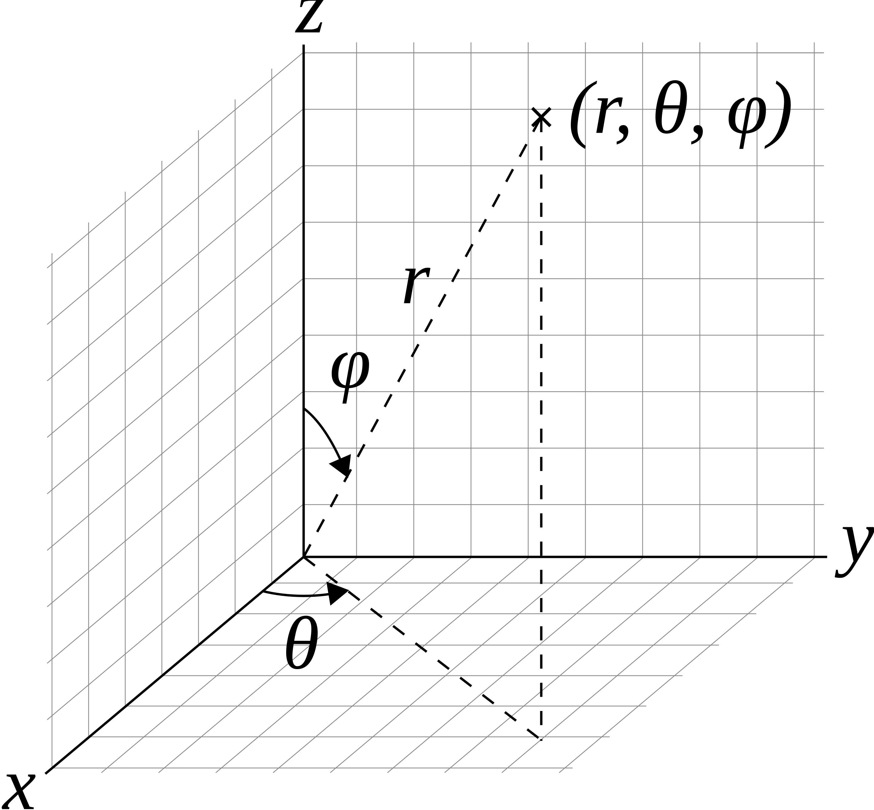
The surface of a sphere can be parametrized by two variables, which are actually angles. Let's assume the sphere is centered on the origin, $\vec{c} = (0, 0, 0)$. Consider the vector from the origin to a point on the sphere, denoted by $\vec{p}$. The first angle is the angle between the z-axis and $\vec{p}$ which is called the polar angle, $\phi$. The second angle is called the azimuthal angle, denoted by $\theta$, and measures the angle from the x-axis to the projection of $\vec{p}$ onto the x-y plane. You can think of this like the angle around the equator.

The range of $\phi$ goes from the north pole to the south pole, which is 180 degrees, or $\pi$ radians: $0 \le \phi \le \pi$. The angle $\theta$ wraps around the entire equator, so $0 \le \theta \le 2\pi$ (360 degrees). For any given $(\theta, \phi)$, we can calculate the (x, y, z) coordinates on the surface of the sphere as:

$$ x = R \sin\phi\cos\theta, \quad y = R\sin\phi\sin\theta, \quad z = R\cos\phi. $$

However, we may wish to switch how $\theta$ and $\phi$ are interpreted, particularly since we have often taken $y$ to be up, and $z$ is pointing towards us (the camera). Either option works, so we just need to be mindful of the geometry in the scene. Assuming we are looking down the $-z$ axis, with the north pole in the $+y$ direction, $\phi$ is now the angle made with the $+y$ axis, and $\theta$ is the angle in the $z$-$x$ plane:

$$ x = R \sin\phi\sin\theta, \quad y = R\cos\phi, \quad z = R\sin\phi\cos\theta. $$

We can also go from $(x, y, z)$ to $(\theta, \phi)$ using:

$$ \theta = \arctan\left(\frac{x}{z}\right) \in [0, 2\pi], \quad \phi = \arccos\left(\frac{y}{R}\right) \in [0, \pi]. $$

Again, these might be different based on your problem setup.

Note that the range of Math.atan2 function is $[-\pi, \pi]$ and the range of Math.acos is $[0, \pi]$. We can almost use this to look up a texture coordinate in an image. We need to apply scaling factors that take into account the range of our angles, as well as the width of the image:

$$ s_{\mathrm{sphere}} = \frac{\texttt{width}}{2\pi}\left(\arctan\left(\frac{x}{z}\right) + \pi\right), \quad t_{\mathrm{sphere}} = \frac{\texttt{height}}{\pi} \arccos\left(\frac{y}{R}\right). $$

where width and height are the width and height of the input texture image (not the dimensions of the destination canvas). We can then use the getImageData function defined for the CanvasRenderingContext2D. For example, this might look like:

  // 1. setup the texture image
  let imgCanvas = document.getElementById("image-canvas");  // replace "image-canvas" with the "id" you assigned to the HTML Canvas
  let imgContext = canvas.getContext("2d", { willReadFrequently: true });
  const img = document.getElementById("earth-texture"); // replace "earth-texture" with the "id" you assigned to your img element
  imgCanvas.width = img.width;
  imgCanvas.height = img.height;
  imgContext.drawImage(img, 0, 0); // draw the image to the canvas so we can look it up

  // 2. loop over pixels:
      // 2a. determine intersection point as usual from ray-scene intersections

      // 2b. calculate s, t from equations above (and round to integers), or use mesh information
      s = ... 
      t = ...

      // 2c. retrieve texture color from img
      const colorData = imgContext.getImageData(s, t, 1, 1);
      color[0] = colorData.data[0] / 255;
      color[1] = colorData.data[1] / 255;
      color[2] = colorData.data[2] / 255;

      // assign 'color' to the pixel
      // ...

This method is a bit slow because we are calling getImageData for each ray-scene intersection, but it highlights the general concept of texturing. We can actually make this a bit more efficient by doing a single call to getImageData to retriave all the texture image data (before the loop over the pixels), and then simply look up the color ourselves. This is how we'll design it in class:

class Texture {
  constructor() {
    this.canvas = document.createElement("canvas");
  }

  texImage2D(image) {
    let context = this.canvas.getContext("2d", {
      willReadFrequently: true,
    });
    this.width = image.width;
    this.height = image.height;
    this.canvas.width = this.width;
    this.canvas.height = this.height;
    context.drawImage(image, 0, 0);
    this.data = context.getImageData(0, 0, this.width, this.height).data;
  }

  texture2D(uv) {
    let us = Math.floor(this.width * uv[0]);
    let vs = Math.floor(this.height * uv[1]);

    let color = vec3.create();
    for (let j = 0; j < 3; j++) {
      const idx = Math.round(this.width * vs + us);
      color[j] = this.data[4 * idx + j] / 255;
    }
    return color;
  }
}

With this utility class, an example of setting up a texture would then be:

let img = document.getElementById("earth-image"); // or whatever image ID you want to use
let texture = new Texture();
texture.texImage2D(img);

This texture can be used to find the color (step 2C above):

const km = texture.texture2D(uv);

These functions might seem like they have strange names, but there is a very specific reason we are calling them texImage2D and texture2D. This is a preview of the WebGL functions we'll use in a few weeks.

More general models: storing an $(s, t)$ value at each vertex.

For more general surfaces represented by a mesh, we don't have an analytic way of getting the $(s, t)$ values. Furthermore, we cannot possibly store every single (s, t) value for points on the surface - we're not even storing every $(x, y, z)$ value of the surface points! Just like we're only storing the $(x, y, z)$ coordinates of each vertex, we'll only store the $(s, t)$ values at each vertex. We can then use interpolation (using barycentric coordinates) to figure out the $(s, t)$ coordinates at a point within each triangle (e.g. from a ray-triangle intersection). The texture coordinates at the vertices can be obtained from the vt lines in an OBJ file.

Revisiting ingredient #3: minification and magnification.

Let's re-interpret our texturing process at the level of a texel. In other words, we are mapping our texel colors to the final pixel. At a certain view, the size of the texel will be exactly the size of the pixel, though this rarely happens. When the surface we are painting is very far away, each pixel we are processing can cover many texel values (size of pixel > size of texel), a phenomenon known as minification. When we are closer to the surface, there may be many texels that map to a single pixel (size of pixel < size of texel), which is known as magnification.

Minification (left) versus Magnification (right) (Interactive Computer Graphics, Angel & Schreiner, 2012)

In the demo below, try to zoom into the chess board (by scrolling the mouse). As we get closer, the effects of magnification start to become apparent, and we can see the "blockiness" (aliasing) in the final image. This is because we were initially using the nearest sample when retrieving a texel. If you change the dropdown to LINEAR, the magnification filter will use a weighted average of the surrounding texels. This is more expensive but will smooth out the blocky artifacts in the image.

The difference between "nearest" and "linear" filters in terms of the magnification problem is also demonstrated in the image below:

Now try scrolling away from the chess board, and notice that the colors don't look as patterned. If you rotate (click and drag) you should also start to see some "flickering" effects. We are now seeing the effects of minification: the texel lookup has many texels to pick from for a single pixel and the one it picks appear somewhat arbitrary. Now change the dropdown to MIPMAP. The chess board should appear to have the correct pattern again, regardless of the distance or how you rotate the square. A mipmap is a minification filter in which a sequence of images is first generated by halving the width and height of the image at each level. Texels will then be looked up at the appropriate level, which can again, use either nearest or linear filters. One disadvantage of mipmaps, however, is that the resulting rendering can look a bit blurry.

Other types of texturing.

Texturing isn't restricted to looking up the color of the surface. We can look up other items that might go into our lighting model. For example, we might want to use an image to look up the normal vector at a point on the surface, or we might want to displace the surface by some amount defined in an image:

normal mapping (a type of bump map): each RGB value in the texture image corresponds to the normal vector $\vec{n} = (n_x, n_y, n_z)$ to be applied in the lighting model. These normals are generally defined in the tangent plane of the surface, so some transformations are necessary to map the normal into physical space.
height mapping (a type of bump map): each RGB value in the texture image (a grayscale image) corresponds to the height perturbation of the surface, from which the normal vector can be recomputed by looking at nearby texels and calculating the gradient. The geometry of the model does not change.
displacement mapping: each RGB value in the texture image corresponds to a displacement of the surface, which actually modifies the geometry. This would be difficult to implement with our ray tracing tools, but is much simpler to do with rasterization (in a few weeks).

It's also possible to look up the specular coefficient (the shininess exponenent $p$ in the Phong Reflection Model) which can produce fingerprint-like effects.

Other texturing methods are also possible such as environment maps (looking up the background image assuming the scene is enclosed in a cube or sphere) and projective texturing, whereby an input image (with known camera orientation and perspective settings) is pasted into our model.

Procedural texturing

Another method for determining the color at a surface point is called procedural texturing, which consists of defining an explicit function (procedure) to describe the relationship between the surface coordinates and the color. This can work using either the 3d surface coordinates or the 2d parametric description of the surface. Note that we already did a form of procedural texturing! Recall Lab 3 when we assigned a kmFunction for BB-8.

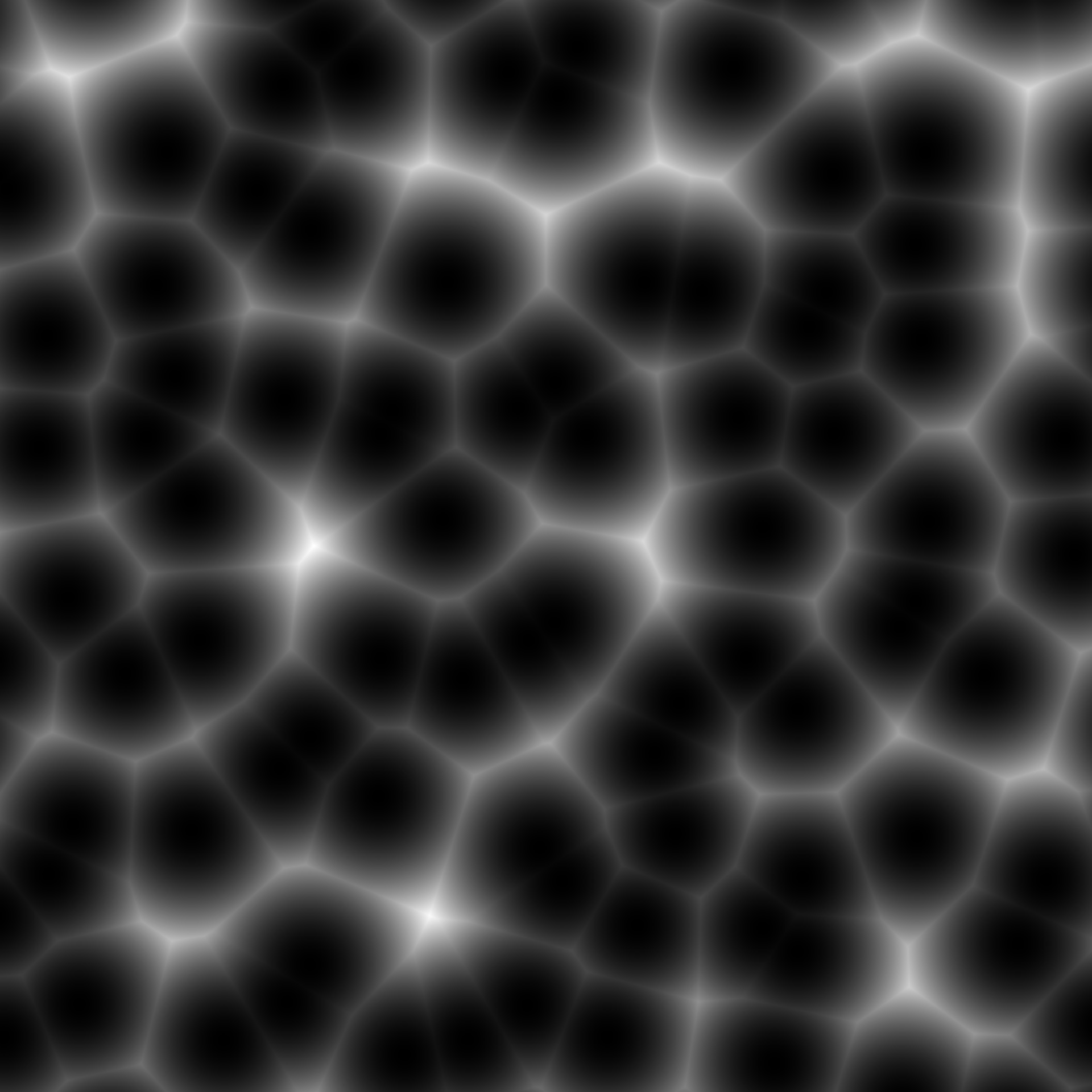
Some of the more popular procedural texturing techniques involve Worley noise (left), Voronoi diagrams (middle) or Perlin noise (right).

A Voronoi pattern can be created by distributing some points (called sites, seeds or generators) on your surface and defining a color for that site. Then, for every ray-surface intersection point, look up the closest site and use the corresponding color of the closest site for your base model color (km). This would make for a great Final Rendering project :)

You'll implement the Perlin noise procedural texturing algorithm in the lab this week. The main idea is to calculate the contributions to the noise from a sequence of grids with random vectors defined at the vertices of the grids (this will be described in detail in the lab).