Chapter 6: Acceleration Structures
Learning Objectives
By the end of this lecture, you will be able to:
- intersect rays with axis-aligned bounding boxes (AABB),
- build a Bounding Volume Hierarchy (BVH) and use it to find ray-model intersections in logarithmic time,
- read
.objfiles.
The bottleneck: intersecting rays with objects.
Our scenes have consisted of a handful of objects (spheres, triangles) so performance hasn't really been an issue yet. But more complex objects require thousands, or even millions of triangles. A for-loop over all of the objects in our scene is very slow. For
An idea: first check if a ray intersects a sphere enclosing the model.
There are a lot of camera rays that never intersect our model, and the pixel color we set to them is just the background sky color. Here's an idea. We know how to intersect rays with spheres, so why don't we enclose our entire model within a sphere and first check if a camera ray intersects this sphere. We'll call this a bounding sphere. If a ray doesn't intersect this sphere, then there's no way it can intersect the model. This means we can already filter out the rays that don't intersect the model and save a loop over many triangles.
This is a good start, but it still lacks some efficiency. What if we are trying to render a giraffe? The model geometry is very long in one direction and very short in another. The bounding sphere of the giraffe will be huge because of the long neck of the giraffe. And there will be a lot of empty space in the sphere between the sides of the giraffe and the surface of the sphere.


A better idea: check if a ray intersects the bounding box enclosing the model.
To make this idea work better, let's try a box instead. We won't use a cube (equal lengths of all sides of the box) because that will have the same issues as the sphere (and probably worse). Instead, we'll find the tightest box around the giraffe and use that as our filter to know if a ray has any chance of intersecting our model.


This type of box is called an axis-aligned bounding box which we will just refer to as an AABB in the rest of the lecture. To define the AABB of our model, we can loop through all the points (each vertex of every triangle) in the model and find the minimum and maximum coordinates, which will define two corners of the box.
Let's define our AABB class that takes in these two corner points:
class AABB {
  constructor(min, max) {
    this.min = min;
    this.max = max;
  }
}
Intersection of a ray with an Axis-Aligned Bounding Box (AABB).
We want to use our AABB of the model to filter out the rays that definitely don't intersect the model. This means we need to know how to intersect rays with boxes. And, actually, we just need to know if a ray intersects a box (not the full intersection information since the box is not something we're going to shade). We know how to do ray-plane intersections (see the Chapter 3 notes), and a box can be interpreted as the intersection of six planes. First, let's represent our ray equation as:
The only difference between this and our previous description is that we're more generally describing the ray origin as
We'll focus on the two planes of the AABB whose normal is aligned with the x-direction:
Similarly for the other constant-x plane (where all points have an x-coordinate of
We then have the interval within which the ray passes between these two planes: min and max to get the correct interval:
It's possible that Infinity in JavaScript). This is actually fine, and our min/max trick will handle this.
The intervals for all x, y and z axes need to overlap.
So we can determine the interval in which a ray intersects the two lower/upper planes in a particular axis direction, but we derived this for infinite planes - it doesn't tell us much about the bounding box. The key observation when applying this idea to the full box is: all three of these
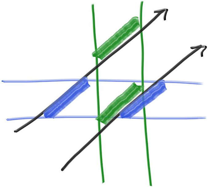
From "Ray Tracing: The Next Week" by Peter Shirley.
In the image above, there are two rays. Rays intersect the bounding box if the green and blue lines overlap. Therefore, in the image above, only the lower ray intersects the bounding box.
For our algorithm, we'll start with an assumption about the valid range of the ray intersection, like
So our intersect function of the AABB class looks like this:
AABB.prototype.intersect = function(ray, tmin, tmax) {
  for (let d = 0; d < 3; d++) {
    // calculate the interval for this dimension
    let tld = Math.min((this.min[d] - ray.origin[d]) / ray.direction[d], (this.max[d] - ray.origin[d]) / ray.direction[d]);
    let tud = Math.max((this.min[d] - ray.origin[d]) / ray.direction[d], (this.max[d] - ray.origin[d]) / ray.direction[d]);
    // update the interval
    tmin = Math.max(tld, tmin);
    tmax = Math.min(tud, tmax);
    // early return if no overlap condition is already satisfied
    if (tmax <= tmin) return undefined; // no intersection with AABB
  }
  return true; // the ray hits this AABB
}
Bounding Volume Hierarchy: A binary tree of bounding boxes.
Great! So we have slightly more efficient way of filtering out whether a ray intersects a model by first checking the bounding box. But it's still not as efficient as it could be. Let's expand upon this idea of bounding boxes.
What if we broke up our model geometry into different pieces, and put a bounding box over each of them. Then, maybe we split up those pieces into smaller pieces, each with a bounding box. For example, maybe we have a bounding box over the giraffe, and break up the giraffe into two pieces: upper body and lower body. Then maybe the upper body is split into one piece for the neck and another for the head, and then maybe the head piece is broken up into a nose, ears, etc. Each of these pieces would have an AABB associated with it (which we can calculate). If a ray does not intersect the upper-body AABB, there's no way it intersects the head AABB, and certainly no way it will intersect the ears. This filters out a lot of triangles to check!

We can represent this using a Bounding Volume Hierarchy, which is a binary tree of these AABBs. In the scene below, the top-level (root) BVH node is labelled as A which has an AABB enclosing all the shapes. A's left child is B which encloses 4 shapes and its right child is C which encloses two shapes.

From Wikipedia.
Building a BVH.
We'll use a top-down approach to building the BVH. For an incoming set of triangles to a particular BVH node, we'll build the two children (left and right) by splitting up the incoming array of triangles into two subarrays. We'll first sort the list according to the coordinates of each triangle along some chosen axis and then put the lower half in the left child and the upper half in the right node. We'll chose this axis randomly, but you can also alternate with each level in the tree (i.e. level % 3). You can also try to find a better split axis which will impact the efficiency of the traversal (for intersections).
Luckily, JavaScript has a built in sorting function for arrays (in-place) and we can pass a custom callback to ask it to sort an array with our own comparator. We'll write a custom comparator that compares two triangles by looking at their lower AABB corner along our random axis:
// Step 1 in BVHNode constructor
const axis = Math.floor(Math.random() * 3);
const compare = (triangleA, triangleB) => {
  return triangleA.box.min[axis] < triangleB.box.min[axis];
}
We'll then slice the incoming array of objects in half when constructing the left and right nodes. Here is the documentation for the Array slice method. Note the end element is not included in the sliced subarray.
We'll also need to handle the cases when there are either 1 or two objects in the incoming objects (triangles) array. These will be the base cases which terminate the BVH construction. When there is only one object, we'll assign it to both the left and right children:
// Step 2 in BVHNode constructor
let nObjects = objects.length;
if (nObjects === 0) {
  return
} else if (nObjects === 1) {
  this.left = objects[0];
  this.right = objects[0];
} else if (nObjects === 2) {
  if (compare(objects[0], objects[1])) {
    this.left = objects[0];
    this.right = objects[1];
  } else {
    this.left = objects[1];
    this.right = objects[0];
  }
} else {
  objects.sort(compare);
  const mid = Math.floor(nObjects / 2);
  this.left = new BVHNode(objects.slice(0, mid));
  this.right = new BVHNode(objects.slice(mid, nObjects));
}
After the left and right children are constructed, we need to give this node an AABB as well since this will be used when we check for intersections. We could loop through all the objects to find the AABB, but this is unnecessary and inefficient. Instead, we'll use the bounding box of the left and right children to determine the bounding box of this node:
// Step 3 in BVHNode constructor
this.box = enclosingBox(this.left.box, this.right.box);
where the enclosingBox function creates a new AABB using the minimum and maximum of the two bounding box coordinates:
const enclosingBox = (boxL, boxR) => {
  const lo = vec3.fromValues(
    Math.min(boxL.min[0], boxR.min[0]),
    Math.min(boxL.min[1], boxR.min[1]),
    Math.min(boxL.min[2], boxR.min[2])
  );

  const hi = vec3.fromValues(
    Math.max(boxL.max[0], boxR.max[0]),
    Math.max(boxL.max[1], boxR.max[1]),
    Math.max(boxL.max[2], boxR.max[2])
  );
  return new AABB(lo, hi);
}
Checking for intersections.
Now we want to use our BVH to check for intersections. As with our earlier ideas, we'll start by checking for an intersection of the root's bounding box with the ray. If no intersection, return undefined as we have been doing:
// Step 1 in BVHNode.prototype.intersect
if (!this.box.intersect(ray, tmin, tmax)) return undefined;
There is a slight difference with how we've been doing object/ray intersections so far. This time, we'll pass in the admissible interval of the ray parameter (tmin and tmax. This will help us filter out whether we need to check a particular branch, as well as define the admissible interval for the AABB intersect method.
If the ray hits the AABB of the current node, first check the left node:
// Step 2 in BVHNode.prototype.intersect
const ixnL = this.left.intersect(ray, tmin, tmax);
If there was a hit, use the resulting t value to bound the check for the right node:
// Step 3 in BVHNode.prototype.intersect
const ixnR = this.right.intersect(ray, tmin, ixnL ? ixnL.t : tmax);
This means we'll automatically ignore any intersection values that are larger than ixnL.t since that wouldn't be the closest anyway. Note that this assumes the object (triangle) eventually returns a ray t value for the intersection, which we have been doing.
If ixnR is not undefined, then we found a closer intersection point than ixnL (if there was one), so we'll prioritize ixnR over ixnL:
// Step 4 in BVHNode.prototype.intersect
return ixnR || ixnL;
Note that a single ray-BVH intersection takes
Other options for speeding up your ray tracer.
Kd-Trees. We built a binary tree representation of our model by dividing the objects (triangles) at each node in the tree. However, we could have also divided the objects by dividing the space along some plane at each node. This is known as a Binary Space Partitioning (BSP) and a special type of BSP is one in which each plane is aligned with a coordinate axis, which is called a Kd-Tree. Kd-Trees are another popular acceleration structure for computer graphics and geometric modeling applications. For more information, please see the pbrt description here.
Parallelization. The camera ray that is sent through a particular pixel does not depend on any information from another pixel. Therefore, our ray tracing algorithm is very well-suited for parallel computation. We could use a multi-threaded approach on the CPU or even write our ray tracer in a language like CUDA or OpenCL for the GPU. Note that NVIDIA has developed the OptiX Ray Tracing Engine for developing ray tracing applications on their GPUs.
OBJ file format
In class, we rendered a giraffe that came from a giraffe.obj file. This was a Wavefront OBJ file which contains information about all the triangles (called a mesh) that represent the giraffe. So far, we have treated triangles as being defined by three 3d points V (real values) and another for the triangle indices T (integer values), which reference the vertices defined in V. This is similar to how you would represent a graph as a collection of vertices and edges in which each edge references two vertices.
In an OBJ file, any line that starts with a v means it is a vertex and the order of the vertices in the file is the same order as they appear in the table V (with indexing starting at 1). Lines that start with f define the indices of the vertices representing a face. For example,
f 1 8 4
defines a triangle (since there are 3 vertex indices listed on this line) which references the first (1), eighth (8) and fourth (4) vertices stored in the V table.
There are other lines that may begin with vt or vn. This allows you to load additional tables and reference either the "vertex texture coordinates" (next week!) or "vertex normals".
Why would we want to load vertex normals? Well, we have talked about computing per-triangle normals, which we can use in our shading models. However, we can also define per-vertex normals and then use the resulting barycentric coordinates from the ray-triangle intersection to interpolate the per-vertex normals. This will produce a smoother-looking shading model. If vertex normals and/or texture coordinates are present in the OBJ file, you might see face descriptors like:
f 1/2/10 4/3/10 5/4/9
There are still three vertices here but the notation a/b/c means a is a vertex coordinate index, b is a reference to a texture coordinate and c is a reference to a vertex normal (all to the corresponding tables). For more information, please see the Wikipedia page on Wavefront OBJ files.
Reading OBJ files with webgl-obj-loader
In class, we used webgl-obj-loader to read OBJ files and then created a bunch of Triangle objects to render (and then possibly create a Bounding Volume Hierarchy from this collection of triangles). The following line in our HTML pages makes the webgl-obj-loader available:
<script src="https://cdn.jsdelivr.net/npm/webgl-obj-loader@2.0.8/dist/webgl-obj-loader.min.js"></script>We can load our mesh with:
const main = (data) => {
  const mesh = data.my_mesh_name; // because of the `my_mesh_name` key defined below

  console.log(mesh.vertices); // this is the V table
  console.log(mesh.indices); // this is the T table

  // set up mesh, BVH, and render...
};

window.onload = () => {
  OBJ.downloadMeshes(
    {
      my_mesh_name: "my_model_file.obj",
    },
    main // the `main` function defined above will run after loading
  );
};
As in Chapter 1, note that mesh.vertices is a one-dimensional array - we need to take a stride of 3 (since the model is in 3d) to access a particular vertex's coordinates. For example, the x, y, and z-coordinates of the fifth (index 4) vertex are:
const vtx = 4; // fifth vertex
const x4 = mesh.vertices[3 * vtx];
const y4 = mesh.vertices[3 * vtx + 1];
const z5 = mesh.vertices[3 * vtx + 2];
The same concept applies to extracting the indices of each triangle, where webgl-obj-loader gives us mesh.indices for these indices. Note that webgl-obj-loader gives us 0-based indices (i.e. a reference index of 1 in the OBJ file will have index 0 in the indices array). For example the three vertex indices of the eight triangle (index 7) are:
const tri = 7;
const t0 = mesh.indices[3 * tri];
const t1 = mesh.indices[3 * tri + 1];
const t2 = mesh.indices[3 * tri + 2];
This means the number of vertices is mesh.vertices.length / 3, and the number of triangles is mesh.indices.length / 3.