CSCI 461: Computer Graphics

Middlebury College, Fall 2023

Lecture 10: Animation 1 (Curves)

Two Modifications to the course structure.

(1) no ShaderToy report, (2) can leave 1 lab in M status for an A.

See changes in blue in course syllabus: https://philipclaude.github.io/csci461f23

We know how to take pictures right now.

How should we create movies?

One option: use physics?

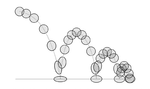
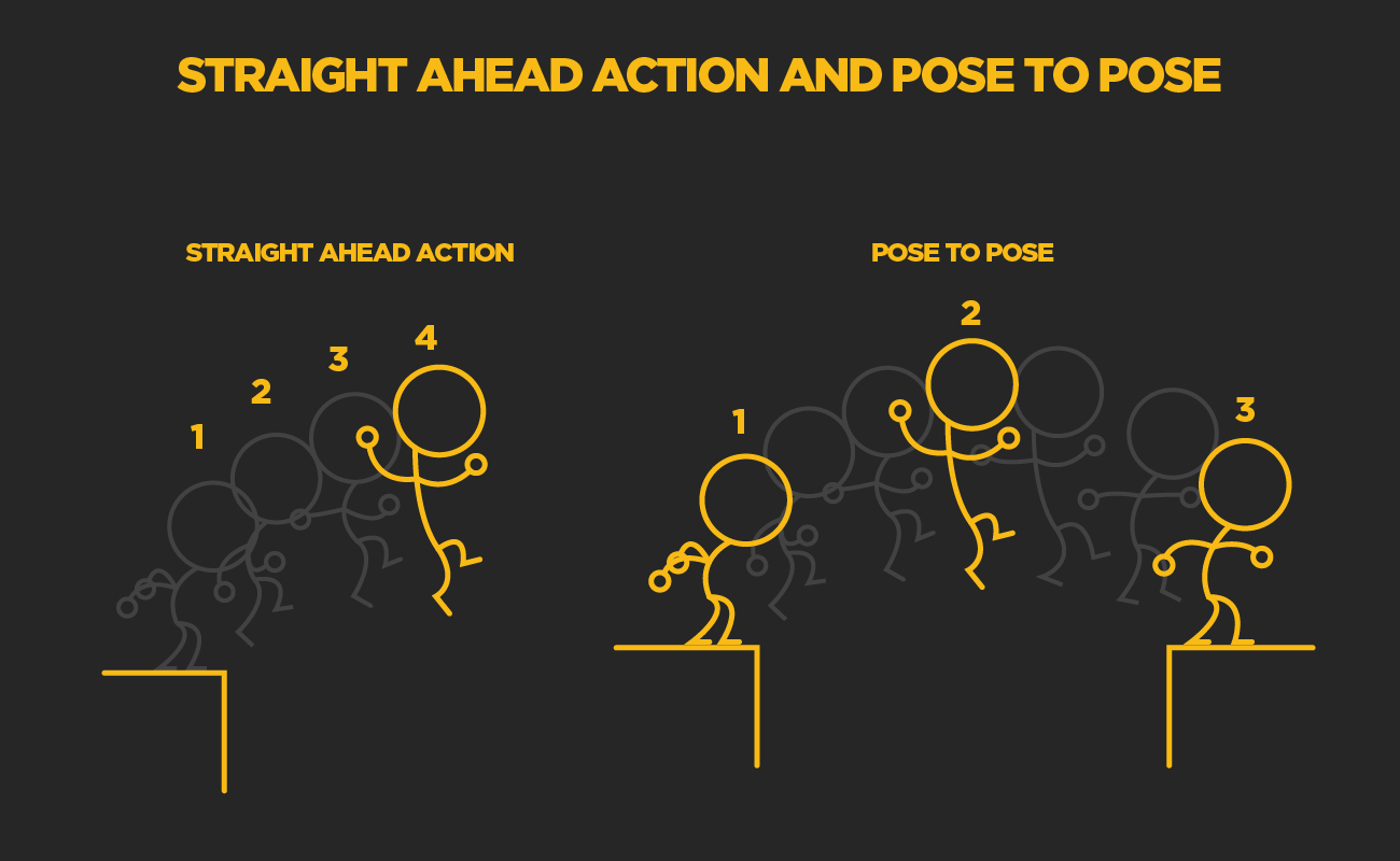
Another option? Let the artist decide.

(source)

Main goal: compute "inbetween" frames by interpolating scene parameters at known frames.

Other things to consider: squash & stretch, timing, slow in and out, arcs (Lasseter, 1987).

By the end of today's lecture, you will be able to:

• specify scene parameters as keyframes in an animation,
• interpolate points to define a smooth curve,
• construct cubic splines from control points,
• represent cubic splines using a Hermite basis and a Bézier basis,
• apply de Casteljau's algorithm to evaluate and render a cubic Bézier curve.

Exercise 1: a few attempts.

Things to be careful of ...

Attempt #3: splines - glue together several curves.

Hermite basis: specify value and derivative at end points.

Solving for coefficients.

$$ y(t) = \left[\begin{array}{cccc} t^3 & t^2 & t & 1 \end{array}\right] \left[\begin{array}{cccc} \phantom{-}2 & -2 & \phantom{-}1 & \phantom{-}1 \\ -3 & \phantom{-}3 & -2 & -1 \\ \phantom{-}0 & \phantom{-}0 & \phantom{-}1 & \phantom{-}0 \\ \phantom{-}1 & \phantom{-}0 & \phantom{-}0 & \phantom{-}0 \end{array}\right] \left[\begin{array}{c} y_{i} \\ y_{i+1} \\ y^\prime_{i} \\ y^\prime_{i+1} \end{array}\right]. $$ And in 2d: $$ \vec p(t) = \left[\begin{array}{cccc} t^3 & t^2 & t & 1 \end{array}\right] \left[\begin{array}{cccc} \phantom{-}2 & -2 & \phantom{-}1 & \phantom{-}1 \\ -3 & \phantom{-}3 & -2 & -1 \\ \phantom{-}0 & \phantom{-}0 & \phantom{-}1 & \phantom{-}0 \\ \phantom{-}1 & \phantom{-}0 & \phantom{-}0 & \phantom{-}0 \end{array}\right] \left[\begin{array}{c} \vec p_{i} \\ \vec p_{i+1} \\ \vec v_{i} \\ \vec v_{i+1} \end{array}\right] $$

Bézier basis: specify 4 controls points of each spline.

Math break!

Combining terms to isolate Bézier basis functions.

$$ \left[\begin{array}{cccc} t^3 & t^2 & t & 1 \end{array}\right] \left[\begin{array}{cccc} -1 & \phantom{-}3 & -3 & \phantom{-}1 \\ \phantom{-}3 & -6 & \phantom{-}3 & \phantom{-}0 \\ -3 & \phantom{-}3 & \phantom{-}0 & \phantom{-}0 \\ \phantom{-}1 & \phantom{-}0 & \phantom{-}0 & \phantom{-}0 \end{array}\right] \left[\begin{array}{c} \vec q_0 \\ \vec q_1 \\ \vec q_2 \\ \vec q_3 \end{array}\right] $$

Properties of Bézier basis functions.

Evaluating a Bézier spline: use basis functions or de Casteljau's algorithm.

Rendering a Bézier spline using de Casteljau's algorithm.

Exercise 2: evaluate and render a curve (by hand!).